You finished CellRanger. CellBender has denoised your 10X output and left you with .h5 files on disk. You now have a count matrix of ~20,000 genes × ~50,000 nuclei across brain regions from 5xFAD Alzheimer mice, and your collaborator wants cluster-level cell types and condition-specific differential expression. The catch: you are doing this on a laptop with 16 GB of RAM, not an HPC node.
Briefly, where those .h5 files come from. In a droplet-based single-cell (or single-nucleus) experiment, tissue is dissociated into a suspension of individual cells — or, for frozen brain, individual nuclei — and each is co-encapsulated with a barcoded bead in its own oil droplet on a 10X Genomics chip. Every transcript inherits a cell barcode (which droplet it came from) and a UMI (which original molecule), so after sequencing the reads can be traced back to a single cell and de-duplicated. CellRanger does that bookkeeping: it aligns reads to the reference genome and produces a genes × cells count matrix. CellBender then removes ambient RNA — free-floating transcripts from lysed cells that contaminate every droplet — yielding cleaner counts. This pipeline deliberately starts after those two steps: alignment and ambient-RNA removal are well-solved, standardised problems, and for GEO datasets like GSE262881 the CellBender-filtered .h5 files are what you download. The analytical decisions that actually shape the biology begin at the count matrix.
Most snRNA-seq tutorials skip the part that actually decides whether the analysis runs at all on consumer hardware — how the count matrix is stored, which normalisation you can afford, and how integration is done. This post is about those three design decisions and the reasoning behind them. The full, runnable implementation already lives in the repository (github.com/SLopezBegines/snRNAseq_mouse); here I explain why it is built the way it is, and where it can still be improved. The pipeline is applied to GSE262881 (Wang et al., BMC Biology 2025).
Why BPCells Is the Decision That Makes the Rest Possible
A dense in-memory representation of a 50k-nuclei dataset is the single biggest reason naïve Seurat pipelines die with cannot allocate vector of size X Gb. Seurat v5 addresses this with BPCells, an on-disk bit-packed sparse matrix backend. Instead of holding the full count matrix in RAM, Seurat operates on a memory-mapped matrix stored on disk and streams only the active subset.
In this pipeline, each CellBender .h5 is written once to an on-disk BPCells directory and reopened from there:
mat_h5 <- BPCells::open_matrix_10x_hdf5(filepath)   # read 10X h5
mat     <- BPCells::write_matrix_dir(mat_h5, dir = bp_dir)  # persist on disk
# on subsequent runs: mat <- BPCells::open_matrix_dir(bp_dir)
The full loader — sample-table parsing from the GEO file-naming convention, per-region filtering, Ensembl→symbol conversion, and checkpointing — is load_h5_samples_bpcells() in code/02_sc_functions.R.
Three consequences follow from this choice, and they propagate through every later step:
- Peak RAM is governed by the largest single operation, not by total dataset size. A 50k-nuclei object that would need ~10 GB dense stays well within 16 GB.
- The matrix is written once and reused. Re-running the notebook reopens the on-disk matrix instead of re-parsing the
.h5, which pairs naturally with the checkpoint system incode/01_aux_functions.R. - Some downstream tools cannot read BPCells directly. This is the cost, and it is the hinge for the next two decisions.
scDblFinder(viaSingleCellExperiment) does not support BPCells, so the pipeline materialises one sample at a time to adgCMatrixfor doublet detection (run_doubletfinder_bp()) — safe at 16 GB precisely because it is per-sample, never the whole dataset at once.
Why LogNormalize, Not SCTransform
This is where the common claim “SCTransform isn’t available in Seurat v5” needs correcting. SCTransform is available in Seurat v5 — you can run SCTransform() and then IntegrateLayers(method = "SCTIntegration"). The reason this pipeline does not use it is practical, not a missing feature.
SCTransform fits a regularised negative-binomial model and, to do so, must materialise the data in memory. It does not operate on a BPCells on-disk matrix the way NormalizeData() (LogNormalize) does in the v5 split-layer workflow. On a 16 GB machine, running SCT means giving back exactly the memory headroom BPCells was introduced to protect — and SCT-based integration in v5 carries additional memory and bookkeeping overhead on top. So the honest statement is: SCT was deliberately not used here because it is incompatible with the on-disk, low-RAM design, not because Seurat v5 lacks it.
LogNormalize, by contrast, is cheap, transparent, and works directly within the split-layer/BPCells workflow:
seurat[["RNA"]] <- split(seurat[["RNA"]], f = seurat$sample_id)
seurat <- NormalizeData(seurat, normalization.method = "LogNormalize", scale.factor = 1e4)
seurat <- FindVariableFeatures(seurat) |> ScaleData() |> RunPCA()
Two further points justify the choice for this dataset specifically. First, the input is already CellBender-denoised, so ambient-RNA-driven depth variation — the regime where SCT’s variance stabilisation helps most — is already reduced upstream. Second, LogNormalize is far easier to audit when a result looks wrong: sequencing-depth effects remain explicit rather than buried inside a fitted model. SCT is the better tool when you have extreme depth variation and the RAM to spare; neither condition holds here. The merge + normalisation logic is in the primary notebook, rmds/snRNAseq_pipeline.qmd.
Why Compare RPCA and Harmony Instead of Picking One
After PCA you still have batch effects — sample-to-sample technical variation that is not biology. Two integration methods dominate, and they make opposite trade-offs:
- RPCA (Reciprocal PCA, the v5 default) is faster and conservative: it corrects fewer batch effects and is less prone to over-correction, but it can leave residual batch structure when effects are strong.
- Harmony corrects in latent space, is more aggressive, and handles strong sample-specific effects well — at the risk of erasing genuine biological differences between conditions.
For GSE262881 (one 5xFAD background, identical handling, CellBender-denoised), batch effects are mild and RPCA is expected to suffice. But “expected to suffice” is a hypothesis, not a result. The pipeline therefore runs both through the same IntegrateLayers() interface and compares them on the same resolution sweep, rather than committing to one a priori:
seurat <- IntegrateLayers(seurat, method = "RPCAIntegration",    new.reduction = "integrated.rpca")
seurat <- IntegrateLayers(seurat, method = "HarmonyIntegration", new.reduction = "integrated.harmony",
                          group.by.vars = "sample_id")
The decision rule is explicit: choose the integration that yields biologically coherent, stable clusters under a clustree resolution sweep (CLUSTERING_DIMS × CLUSTERING_RESOLUTIONS, set in code/global_variables.R) — not the one that produces the most clusters. With strong over-correction, real Ctrl-vs-Inulin differences would collapse; that failure mode is exactly what comparing the two methods is designed to catch.
Where the Reasoning Pays Off Downstream
The QC, doublet, clustering and annotation stages are unchanged in logic from the modular scripts and are documented in the repo, so I will not repeat the code here. Two principles carry through: everything that can be done per-sample is done per-sample before merging (QC thresholds, doublet detection), because merging first leaks cross-sample bias; and automated annotation is a first pass, never the final word. SingleR (Allen Brain Atlas / MouseRNAseqData) gives a label; canonical markers and per-cluster DE decide whether to trust it.
The annotated output, at resolution 0.5 for GSE262881:
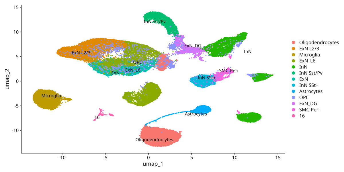 Annotated UMAP (forebrain + cerebellum, 5xFAD mouse, ~50k nuclei): excitatory and inhibitory neuron subtypes, oligodendrocytes, OPC, astrocytes, microglia, SMC-pericytes, and one unresolved cluster (16) left deliberately unlabeled. Don’t rename ambiguous clusters — document and investigate them.
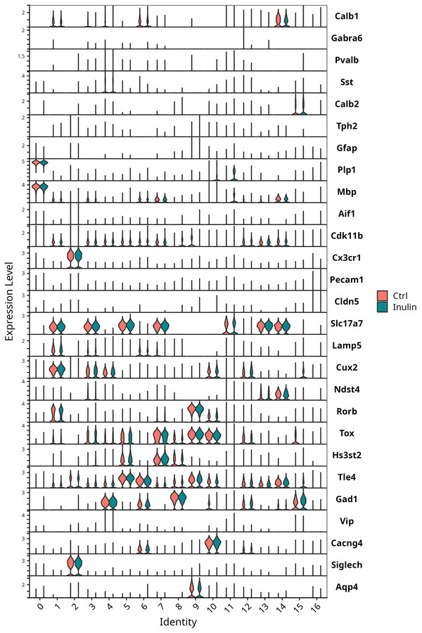 Split VioinPlot of canonical markers across clusters (Ctrl / Inulin). This is the manual-validation step that SingleR alone cannot replace.
Per-cluster GO/GSEA (clusterProfiler::gseGO()) then gives a functional read per cell population — run per cluster, not on a single global DE list, so that distinct signatures (e.g. mitochondrial activation in interneurons vs. DAM genes in microglia) are not averaged away.
Limitations and Planned Improvements
Being explicit about what this pipeline does not yet do is part of the methodology:
- No formal integration metric. The RPCA-vs-Harmony choice is currently made by visual inspection of UMAP +
clustree. A quantitative score (kBET, LISI/iLISI, orscIBmetrics) would make the decision reproducible rather than judgement-based. - Wilcoxon DE ignores the sample hierarchy.
FindMarkerstreats nuclei as independent, which inflates significance. Pseudobulk DE (aggregate counts per sample, thenDESeq2/edgeR) is the more defensible test for condition contrasts and is the main planned upgrade. - scDblFinder requires per-sample materialisation. A doublet method that reads BPCells natively would remove the one place the on-disk design is broken.
- SingleR reference is generic. A region-matched brain reference (e.g. Allen taxonomy at finer resolution) would improve subtype calls.
- Scaling ceiling. Beyond ~50k nuclei even BPCells + sequential
futureslows;SketchIntegration(sketch-based) is the v5 route worth testing next.
Conclusion
The three decisions that define this pipeline are coupled, not independent. BPCells makes a 50k-nuclei analysis fit in 16 GB; that choice rules out SCTransform (which would force the data back into memory) and points to LogNormalize; and because no single integration method is universally correct, RPCA and Harmony are compared rather than assumed. None of this is exotic — it is the result of taking the hardware constraint seriously and letting it propagate honestly through the method.
Full code, the GSE262881 analysis, and the modular scripts referenced above: github.com/SLopezBegines/snRNAseq_mouse.
References
-
Seurat v5: Hao Y. et al. (2024). Dictionary learning for integrative, multimodal and scalable single-cell analysis. Nature Biotechnology 42, 293–304. doi:10.1038/s41587-023-01767-y
-
BPCells: on-disk bit-packed sparse matrix backend for single-cell data, integrated with Seurat v5. Software: github.com/bnprks/BPCells
-
SCTransform: Hafemeister C. & Satija R. (2019). Normalization and variance stabilization of single-cell RNA-seq data using regularized negative binomial regression. Genome Biology 20, 296. doi:10.1186/s13059-019-1874-1
-
RPCA integration: Hao Y. et al. (2021). Integrated analysis of multimodal single-cell data. Cell 184(13), 3573–3587. doi:10.1016/j.cell.2021.04.048
-
Harmony integration: Korsunsky I. et al. (2019). Fast, sensitive and accurate integration of single-cell data with Harmony. Nature Methods 16, 1289–1296. doi:10.1038/s41592-019-0619-0
-
CellBender: Fleming S.J. et al. (2023). Unsupervised removal of systematic background noise from droplet-based single-cell experiments using CellBender. Nature Methods 20, 1323–1335. doi:10.1038/s41592-023-01943-7
-
scDblFinder: Germain P.-L. et al. (2022). Doublet identification in single-cell sequencing data using scDblFinder. F1000Research 10, 979. doi:10.12688/f1000research.73600.2
-
SingleR: Aran D. et al. (2019). Reference-based analysis of lung single-cell sequencing reveals a transitional profibrotic macrophage. Nature Immunology 20, 163–172. doi:10.1038/s41590-018-0276-y
-
clusterProfiler: Wu T. et al. (2021). clusterProfiler 4.0: A universal enrichment tool for interpreting omics data. Innovation 2(3), 100141. doi:10.1016/j.xinn.2021.100141
-
Dataset: Wang X. et al. (2025). A single-cell transcriptomic atlas of all cell types in the brain of 5xFAD Alzheimer mice in response to dietary inulin supplementation. BMC Biology 23, 124. doi:10.1186/s12915-025-02230-x · GEO: GSE262881
About the author: Santiago López Begines is a PhD-trained neuroscientist and data scientist specialising in omics data pipelines, biomarker discovery, and quantitative proteomics. For scientific collaborations or methodological exchanges, get in touch.