Label-free quantitative (LFQ) proteomics measures protein abundance directly from mass spectrometry signal intensity. It’s powerful, but messier than other omics: proteins disappear from the dataset when they fall below the instrument’s detection limit or when sampling variance prevents quantification in particular replicates, or can also depends of detection method (DDA vs. DIA). The result is a dataset riddled with missing values—and how you handle them shapes your downstream statistical conclusions.
This post walks through the problem, the theory behind different imputation mechanisms, and a practical mixed-strategy implementation in R that adapts the method to the missing data pattern observed in each protein-condition combination.
The Missing Data Problem in LFQ Proteomics
In a typical LFQ experiment, you have a matrix with proteins as rows and biological samples (usually grouped by experimental condition and replicate) as columns. The cells contain log-transformed intensity values. But many cells are NA—sometimes 30%, 50%, or more, depending on detection sensitivity and experimental noise.
Why does this happen?
- Stochastic sampling: Even abundant proteins may randomly fail to ionize in a given MS run. This is rare for highly abundant proteins, but common for proteins near the median abundance range.
- Detection limit: Proteins with abundance below the instrument’s threshold never appear. If a protein is genuinely absent or extremely low in one condition but present in another, it will be missing only in the low condition.
- Sample preparation variability: Protein extraction, quantification, and normalization introduce run-to-run variance. A protein just barely above threshold in one sample may drop below it in another due to batch effects.
The critical insight: missing values in proteomics maybe not random. They cluster in proteins with low abundance, and they can be biased toward specific conditions. This matters because most statistical tests assume complete data, and naive imputation (like replacing NAs with zero or the global median) introduces bias.
Understanding Missing Data Mechanisms: MCAR, MAR, and MNAR
Rubin’s framework12 classifies missing data into three categories:
Missing Completely At Random (MCAR)
The probability that a value is missing is independent of both the observed and unobserved values. Example: a pipetting error that randomly ruins one well has nothing to do with the protein’s true abundance.
In practice, MCAR is rare in proteomics (and to be honest, MCAR are difficult to discern from MAR).
Missing At Random (MAR)
The probability of missingness depends on observed values but not on the missing value itself. Example: a protein is missing in replicate A because its abundance is systematically lower in condition A (observed in other samples), but the mechanism is not specific to condition A. Randomness from detection method, preprocessing of sample (precipitation, digestion, normalization….)
For MAR data, the missing mechanism is ignorable under the right model, and methods like k-nearest neighbors (kNN) or maximum likelihood work well.
Missing Not At Random (MNAR)
The probability of missingness depends on the unobserved value itself. Example: a protein is missing in condition B because its abundance is below the detection limit in that condition—we don’t know it’s low; we only know it’s systematically absent in that condition. The missingness directly reveals information about the missing value (it’s very low).
MNAR is the dominant pattern in label-free proteomics. Proteins missing in all replicates of a condition are likely at or below the detection limit in that condition. Using kNN to impute from other samples where the protein is present would incorrectly assume the protein is abundant enough to measure but happened to be missed—a violation of the MAR assumption.
A Visual Diagnostic
Before imputing, you should always plot the missing value pattern. This repo LFQ proteomic analysis pipeline & blog entry (LFQ Proteomics project) are based on DEPpackage (version 1.32.0) from Bioconductor. All code presented here can be found at Mixed imputation script. The DEP R package generates a heat-map showing which proteins and samples have missing values. Patterns you’ll see:
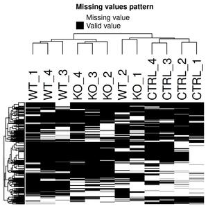
- Vertical stripes: A sample has many missing values (possible batch effect or low protein recovery).
- Horizontal stripes: A protein is missing across many or all samples (likely a true absence or very low abundance).
- Block patterns: A protein is missing in one condition but not others (strong sign of MNAR—the protein is condition-specific or below detection in that condition).
The Mixed-Strategy Approach
This is based on official documentation of DEP package: Missing value handling
The solution is to classify each protein per condition as either MAR or MNAR, then apply the appropriate imputation method to each subset. Here’s the logic:
MNAR classification rule: A protein is MNAR in a given condition if it is missing in ≥ fraction_NA fraction of replicates in that condition. (Default: ≥ 60%.). In this example, with 4 replicates any 0.5 < fraction_NA < 0.75 would work in the same way.
Why? If a protein is missing in 3 out of 4 replicates of condition A, it’s almost certainly below detection in condition A. If it’s missing in only 1 out of 4, it could be stochastic (MAR).
Imputation for MNAR proteins: Ideally, the use of a left-censored method is recomended. In practice, this imputation method fail when there are too missing values for a protein in a given condition (i.e. knocked-out protein in KO condition). The script uses impute(..., fun="zero") to impute “zero” value to this samples. This similar what is done in the official documentation, but in this case, we replace “zero” with a truncated left-censored distribution (truncnorm::rtruncnorm()) centered around value_impute, with upper truncation in the global minimum and a spread of 0.3 (matching the # ‘scale’ parameter of MSnbase::impute(fun = “man”)) .
global_min <- min(assay(data_norm), na.rm = TRUE)
value_impute <- global_min - sd(assay(data_norm), na.rm = TRUE) * factor_SD_impute
Why this is statistically correct
The left-censored model assumes: proteins are present but below the detection threshold, so their true intensities live in the tail of the overall distribution that was cut off at measurement. rtruncnorm(…, b = global_min) samples exactly from that unobserved tail, centered at value_impute with configurable spread — matching what MinProb/man do internally, but anchored at your explicit value_impute instead of a quantile-derived center.
With this left-censored distribution, we avoid to apply the same artificial value below detection limit to al MNAR, what could kills variability, and create artificial clustering in PCA.
Imputation for MAR proteins: Use kNN. The script applies impute(..., fun="knn", rowmax=0.9), which imputes each missing value as the average of the k nearest proteins (by Euclidean distance in the current condition subset). This preserves the covariance structure among proteins.
Implementation in R
Here’s the key section of the mixed imputation pipeline:
  ### Mixed Condition-Splited ####
  # Strategy: classify each protein-per-condition independently as MNAR or MAR.
  # A protein is MNAR in a given condition if it is missing in >= fraction_NA
  # of replicates of that condition — indicating it is near/below the detection
  # limit rather than stochastically absent.
  #
  # MNAR imputation uses a two-step approach:
  #   1. MSnbase::impute(mnar = "zero") sets MNAR NAs → 0 as a placeholder.
  #   2. Those zeros are then replaced with draws from a left-truncated Gaussian:
  #        N(mean = value_impute, sd = sd_scale) truncated above at global_min.
  #      Truncating at global_min guarantees every imputed value falls below the
  #      observed detection floor, consistent with the left-censored MNAR model.
  #      Using a distribution (not a fixed scalar) preserves variability among
  #      MNAR proteins, preventing artificial clustering in PCA and spikes in the
  #      intensity histogram.
  #
  # MAR proteins are imputed with kNN using observed values from other samples.
  # This per-condition split avoids over-imputation of true absences with kNN.

  # 1. Create the MNAR flag table from the long-format data.
  proteins_MNAR <- get_df_long(data_norm) %>%
    mutate(across(where(is_character), as_factor)) %>%
    group_by(name, condition) %>%
    summarize(
      frac_NA = sum(is.na(intensity)) / n(), # fraction of missing values
      num_NAs = sum(is.na(intensity)), # absolute count of missing values
      MNAR_flag = frac_NA >= fraction_NA, # TRUE → treat as left-censored (MNAR)
      .groups = "drop"
    )

  # save proteins_MNAR as xlsx
  write.xlsx(proteins_MNAR, paste0(output_path, "tables/proteins_MNAR_", name_df, ".xlsx"))


  # 2. Get the unique conditions from the SummarizedExperiment metadata.
  #    We assume that colData(data_norm)$condition exists.
  conditions <- unique(colData(data_norm)$condition)
  # Global minimum for left-censored distribution
  global_min <- min(assay(data_norm), na.rm = TRUE)
  value_impute <- global_min - sd(assay(data_norm), na.rm = TRUE) * factor_SD_impute
  # Spread of the truncated-normal draws: a fraction of the global SD.
  # Default 0.3 matches the 'scale' parameter of MSnbase::impute(fun = "man").
  sd_scale <- sd(assay(data_norm), na.rm = TRUE) * factor_SD_scale
  # 3. Process each condition separately so the MNAR/MAR classification is
  #    condition-specific. A protein absent only in one condition should be
  #    MNAR-imputed in that condition but kNN-imputed (MAR) in others.
  imputed_list <- lapply(conditions, function(cond) {
    # Subset to samples belonging to this condition only.
    se_cond <- data_norm[, colData(data_norm)$condition == cond]

    # Build a per-protein logical vector for impute():
    #   randna = TRUE  → protein is MAR → use kNN
    #   randna = FALSE → protein is MNAR → use left-censored method (mnar = "zero")
    # MNAR_flag = TRUE means ≥ fraction_NA missing → randna must be FALSE (not random).
    randna_vec <- sapply(rownames(se_cond), function(prot) {
      flag <- proteins_MNAR %>%
        filter(name == prot, condition == cond) %>%
        pull(MNAR_flag)
      if (length(flag) == 0) {
        # If no record is found, assume MAR.
        return(TRUE)
      } else {
        # If MNAR_flag is TRUE (i.e. high missingness) then we want zero imputation,
        # so set randna (MAR flag) to FALSE.
        return(!flag)
      }
    })

    # Sanity check: ensure we have one flag per protein.
    if (length(randna_vec) != nrow(se_cond)) {
      stop("Mismatch in protein numbers for condition: ", cond)
    }

    # Perform the mixed imputation on this condition subset.
    imputed_se <- impute(se_cond,
      fun = "mixed",
      randna = randna_vec, # vector for this condition
      mar = "knn", # imputation method for MAR values
      mnar = "zero" # imputation method for MNAR values
    ) # imputation method for MNAR values
    return(imputed_se)
  })


  # 4. Combine the imputed data back together.
  #    Here, we assume that the protein order is the same across conditions.
  #    We combine the assays (columns) from each condition subset.
  imputed_assays <- lapply(imputed_list, assay)
  imputed_matrix <- do.call(cbind, imputed_assays)

  # Replace zeros (MNAR placeholders) with draws from a left-truncated Gaussian.
  #
  # Why truncated normal instead of a fixed scalar?
  #   - A plain Gaussian centered at value_impute can produce draws above global_min,
  #     contaminating the observed intensity range with imputed noise.
  #   - rtruncnorm(..., b = global_min) truncates the distribution at the detection
  #     floor so every draw is guaranteed to be below the observed minimum, consistent
  #     with the left-censored MNAR assumption.
  #   - Using a distribution (rather than a fixed scalar) preserves variability among
  #     MNAR proteins, preventing artificial clustering in PCA and intensity spikes.
  #
  # Distribution parameters:
  #   mean = value_impute  = global_min - factor_SD_impute * sd  (center, below detection floor)
  #   sd   = sd_scale      = factor_SD_scale * sd                (spread, default 0.3 × sd)
  #   b    = global_min                                          (upper truncation point)
  n_zeros <- sum(imputed_matrix == 0)
  imputed_matrix[imputed_matrix == 0] <- truncnorm::rtruncnorm(
    n    = n_zeros,
    a    = -Inf,
    b    = global_min, # upper bound: no imputed value can exceed the detection floor
    mean = value_impute, # center: factor_SD_impute SDs below global minimum
    sd   = sd_scale # spread: factor_SD_scale fraction of global SD (default 0.3)
  )

  # 5. Replace the assay in the original SummarizedExperiment with the imputed matrix.
  #    This creates a new SummarizedExperiment with imputed data.
  mixed_splited_imputation <- data_norm
  assay(mixed_splited_imputation) <- imputed_matrix

  proteins_MNAR <- proteins_MNAR %>%
    pivot_wider(
      names_from = condition,
      values_from = c(frac_NA, MNAR_flag, num_NAs),
      names_sep = "_"
    ) %>%
    dplyr::rename(genename = name)
  # Now, add proteins_MNAR as aditional metadata:
  metadata(mixed_splited_imputation)$proteins_MNAR <- proteins_MNAR
The MSnbase::impute() function (from the Bioconductor MSnbase package) is the workhorse here. The fun="mixed" argument accepts a logical vector (randna) specifying which proteins should use random imputation (MAR) versus deterministic left-censored imputation (MNAR).
Quality Control: Checking That Imputation Preserves Variance Structure
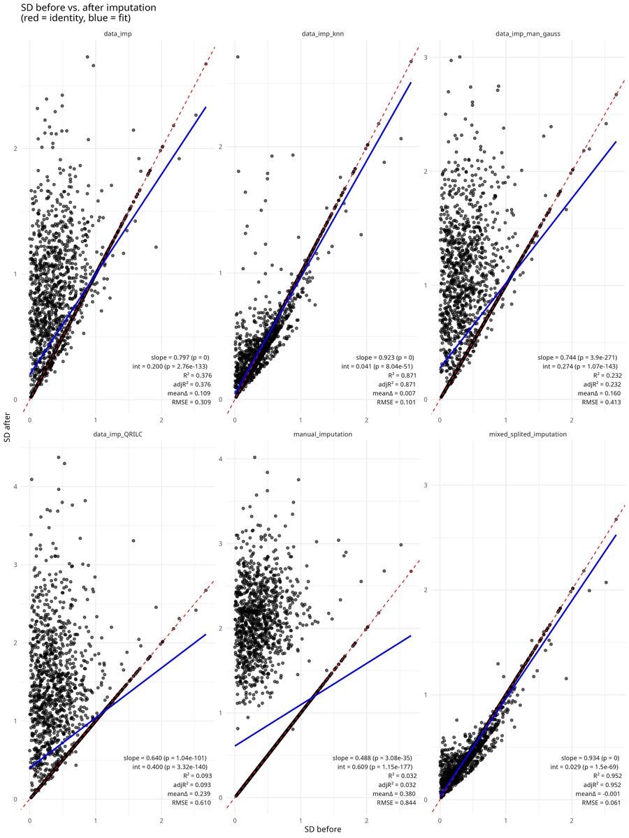
A good imputation should not drastically inflate or deflate per-protein standard deviation. If it does, it can bias downstream statistical tests (e.g., inflate false positives if it artificially reduces variance).
The script includes a diagnostic function that compares standard deviation before and after imputation for each method:
  # compare_sd_imputations() ----------------------------------------------
  # Diagnostic: compare per-protein SD before and after imputation for each
  # method. A good imputation should preserve the pre-imputation SD structure
  # (slope ≈ 1, intercept ≈ 0 in the before-vs-after scatter). Methods that
  # severely inflate or deflate SD distort the downstream limma model.
  # Exports a scatter plot, a wide SD table, and a linear model summary per method.
  # ----------------------------------------------------------------------- #
  compare_sd_imputations <- function(data_norm, impute_list, output_path) {
    # 1) SD before
    sd_before_df <- get_df_long(data_norm) %>%
      mutate(across(where(is.character), as_factor)) %>%
      group_by(name, condition) %>%
      summarize(
        sd_before = sd(intensity, na.rm = TRUE),
        .groups   = "drop"
      )

    # 2) SD after, for each imputed object
    sd_after_df <- bind_rows(
      lapply(names(impute_list), function(meth) {
        get_df_long(impute_list[[meth]]) %>%
          mutate(across(where(is.character), as_factor)) %>%
          group_by(name, condition) %>%
          summarize(
            sd_after = sd(intensity, na.rm = TRUE),
            .groups  = "drop"
          ) %>%
          mutate(method = meth)
      })
    )

    # 3) join before & after
    var_df <- sd_after_df %>%
      left_join(sd_before_df, by = c("name", "condition"))

    # 4) wide table of per‐protein SDs
    var_df_wide <- var_df %>%
      pivot_wider(
        id_cols = c(name, condition, sd_before),
        names_from = method,
        values_from = sd_after,
        names_prefix = "sd_after_"
      )
    assign("var_df_wide", var_df_wide, envir = .GlobalEnv)

    # export wide SD table
    dir.create(file.path(output_path, "tables"), recursive = TRUE, showWarnings = FALSE)
    write.xlsx(
      var_df_wide,
      file = file.path(output_path, "tables", "SD_before_after_imputation.xlsx"),
      overwrite = TRUE
    )
    print(var_df_wide)

    # 5) Build per‐method lm summaries and deviation metrics
    metrics_df <- var_df %>%
      filter(!is.na(sd_before), !is.na(sd_after)) %>%
      group_by(method) %>%
      nest() %>%
      mutate(
        model     = purrr::map(data, ~ lm(sd_after ~ sd_before, data = .x)),
        glance    = purrr::map(model, broom::glance),
        tidy_coef = purrr::map(model, broom::tidy)
      ) %>%
      unnest_wider(glance, names_sep = "_") %>%
      unnest(tidy_coef) %>%
      filter(term %in% c("(Intercept)", "sd_before")) %>%
      select(
        method,
        term,
        estimate,
        p.value,
        glance_r.squared,
        glance_adj.r.squared
      ) %>%
      pivot_wider(
        names_from  = term,
        values_from = c(estimate, p.value),
        names_glue  = "{term}_{.value}"
      ) %>%
      rename(
        intercept     = `(Intercept)_estimate`,
        slope         = sd_before_estimate,
        p_intercept   = `(Intercept)_p.value`,
        p_slope       = sd_before_p.value,
        r_squared     = glance_r.squared,
        adj_r_squared = glance_adj.r.squared
      ) %>%
      left_join(
        var_df %>%
          mutate(delta_sd = sd_after - sd_before) %>%
          group_by(method) %>%
          summarize(
            mean_delta = mean(delta_sd, na.rm = TRUE),
            rmse       = sqrt(mean(delta_sd^2, na.rm = TRUE)),
            .groups    = "drop"
          ),
        by = "method"
      ) %>%
      mutate(
        label = sprintf(
          "slope = %.3f (p = %.3g)\nint = %.3f (p = %.3g)\nR² = %.3f\nadjR² = %.3f\nmeanΔ = %.3f\nRMSE = %.3f",
          slope, p_slope,
          intercept, p_intercept,
          r_squared,
          adj_r_squared,
          mean_delta,
          rmse
        )
      )

    # write out the enhanced summary
    write.xlsx(
      metrics_df %>% select(-label),
      file = file.path(output_path, "tables", paste0(
        "fraction_NA_", fraction_NA,
        "_factor_SD_impute_", factor_SD_impute,
        "_SD_imputation_summary.xlsx"
      )),
      overwrite = TRUE
    )
    print(metrics_df)

    # 6) scatter + annotations
    p1 <- ggplot(var_df, aes(x = sd_before, y = sd_after)) +
      geom_point(alpha = 0.6) +
      geom_abline(
        slope = 1, intercept = 0,
        color = "red", linetype = "dashed"
      ) +
      geom_smooth(method = "lm", se = FALSE, color = "blue") +
      facet_wrap(~method, scales = "free") +
      geom_text(
        data = metrics_df,
        aes(x = Inf, y = -Inf, label = label),
        hjust = 1.1,
        vjust = -0.2,
        size = 3,
        inherit.aes = FALSE
      ) +
      labs(
        title = "SD before vs. after imputation\n(red = identity, blue = fit)",
        x     = "SD before",
        y     = "SD after"
      ) +
      theme_minimal()

    save_plot("%02d_SD_before_after_scatter", p1,
      output_dir = paste0(output_path, "figures"),
      width = 12, height = 16
    )
  }

  # Example usage:
  imputation_list <- list(
    data_imp = data_imp,
    data_imp_man_gauss = data_imp_man_gauss,
    data_imp_knn = data_imp_knn,
    mixed_splited_imputation = mixed_splited_imputation,
    manual_imputation = manual_imputation,
    data_imp_QRILC = data_imp_QRILC
  )
  compare_sd_imputations(data_norm, imputation_list, output_path)
Scatter plots of SD before vs. after, with regression lines and slope/intercept annotations, reveal which methods preserve the variance structure best. This is crucial for selecting an imputation approach.
Practical Recommendations
-
Always visualize your missing data. Use heatmaps and intensity-distribution plots to understand the pattern. Is it random, condition-specific, or abundance-dependent?
-
Use a mixed strategy. Don’t apply a single imputation method to all proteins. Proteins with few missing values (likely MAR) should be handled differently from proteins with many missing values (likely MNAR).
-
Classify missingness conservatively. Set
fraction_NA(the threshold for calling a protein MNAR) based on your replicate count. With 4 replicates, 0.5–0.6 is reasonable. With 3 replicates, 0.67 may be too high; consider 0.5. -
Use a left-censored method for MNAR. MinProb, QRILC, or manual Gaussian imputation all work; choose based on your intensity distribution. The script offers all three.
-
For MAR, use kNN or a model-based method. kNN preserves covariance structure. Maximum likelihood (e.g., MLE in MSnbase) is more principled but computationally heavier.
-
Check that imputation doesn’t distort variance. Generate SD-before-vs.-after plots. If imputation inflates variance in low-abundance proteins, you may have used too many near-minimum values; if it deflates, you may have over-smoothed.
-
Test sensitivity. Run differential abundance analysis on multiple imputation strategies and compare the number of significant proteins recovered. If results are robust, your choice of imputation matters less. If they differ dramatically, investigate the mechanism.
-
Document your choices. Report the fraction_NA threshold, imputation methods, and the number of proteins classified as MNAR vs. MAR. Future readers (including your future self) will appreciate this detail.
Conclusion
Missing data imputation in label-free proteomics is not one-size-fits-all. The mixed-strategy approach—classifying missingness per protein and condition, then applying MNAR or MAR methods accordingly—is more robust than global imputation and reflects the underlying biology of your data. The R implementation shown here, wrapped in the data_cleaning() function, scales to large cohorts and includes built-in quality control diagnostics to validate your choices.
Use this as a template for your own proteomics pipelines. Adjust the fraction_NA, factor_SD_scale and factor_SD_impute parameters based on your instrument, sample preparation, and replicate design. Always visualize; always validate.
About the author: Santiago López Begines is a PhD-trained neuroscientist and data scientist specializing in omics data pipelines, biomarker discovery, and quantitative proteomics. This post draws on production code from his Proteomics analysis suite, available in his GitHub repositories. For colaboration in bioinformatics or statistical analysis, get in touch.
-
Rubin, D. B. (1976). Inference and Missing Data. Biometrika, 63(3), 581–592. https://doi.org/10.1093/biomet/63.3.581 ↩
-
Carpenter, J. R., & Smuk, M. (2021). Missing Data: A Statistical Framework for Practice. Biometrical Journal, 63(5), 915–947. https://doi.org/10.1002/bimj.202000196 ↩