You have a count matrix: rows are genes, columns are samples, each cell is a read count. You want to know what changed between conditions. Before you call anything “significant,” you make a chain of decisions — which statistical model, how to handle the variance structure, how to shrink fold-change estimates, how much to trust a single method — and each one compounds. Get them wrong and you either miss real signal or publish noise.
This post is about three of those decisions, applied to GSE168137: a 192-sample 5xFAD Alzheimer mouse dataset (Forner et al., Scientific Data 2021) covering four timepoints (4, 8, 12, 18 months), two brain regions (cortex and hippocampus), and both sexes. The full, modular implementation lives in the repository (github.com/SLopezBegines/bulkRNAseq); here I explain the reasoning and show what the data said — including why the headline result is a starting point, not a conclusion.
Briefly, where the counts come from. In bulk RNA-seq, RNA is extracted from a whole tissue sample, reverse-transcribed, sequenced, and the reads aligned and tallied per gene. Unlike single-cell, there is no per-cell resolution: every count is the average expression across all the cells in that sample, dominated by whatever cell types are most abundant. That averaging is the method’s strength (stable, deep, cheap) and its limitation (it cannot tell you which cell type changed). The analysis below starts at the count matrix GEO provides as GSE168137_countList.txt.gz.
The Experimental Design
GSE168137 is a fully crossed factorial design built to phenotype the 5xFAD model systematically rather than at a single endpoint. The 5xFAD line carries five familial AD mutations and develops progressive amyloid pathology; wild-type C57BL/6J (BL6) littermates are the controls. Four factors are crossed:
| Factor | Levels |
|---|---|
| Genotype | 5xFAD (transgenic) vs BL6 (wild-type) |
| Tissue | Cortex, Hippocampus |
| Age | 4, 8, 12, 18 months |
| Sex | Female, Male |
| Samples | 192 total |
The count matrix is gene-level, aligned to GRCm38 with Ensembl IDs (version suffix stripped), and starts at 55,449 features across the 192 samples before filtering. The crossed structure is what makes the analysis interesting and what makes the design formula consequential: genotype is only one of four factors moving at once, and three of them (tissue, age, sex) are nuisance variation for the 5xFAD-vs-BL6 question. The contrast tested throughout is 5xFAD vs BL6, with the other factors handled in the model rather than ignored.
Decision 1: The Design Formula — And Why Tissue Changes Everything
The most consequential line in a DESeq2 analysis is the design formula. The common mistake is to test only the variable of interest:
design = ~ genotype # tests 5xFAD vs BL6 — and nothing else
This is valid only if every other source of variation is held constant. GSE168137 is a full factorial: 2 genotypes × 2 regions × 4 timepoints × 2 sexes. Ignore those and you treat a 4-month female cortex sample as interchangeable with an 18-month male hippocampus sample. The nuisance variance leaks into the genotype estimate, standard errors shrink artificially, and p-values become anti-conservative — false positives.
The fix is to put confounders in the formula so they absorb variance you do not care about. The reported run uses:
design = ~ sex + age_months + genotype + tissue # genotype is the term of interest
But which confounders? That is an empirical question, and the data answers it. Running PCA on the top 500 variable VST-normalised genes (code/06_dimreduction.R) shows the dominant axis of variation is not genotype:
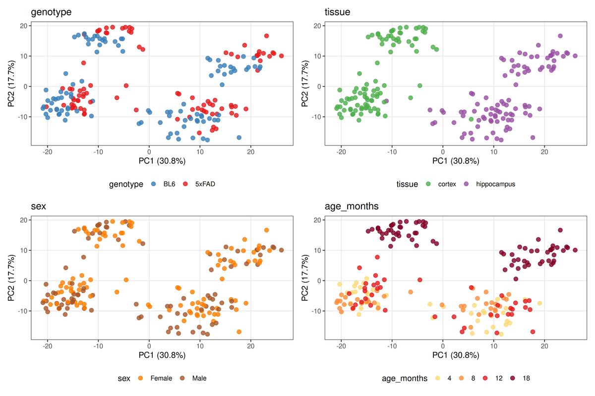 PCA of 192 samples (PC1 = 30.8%, PC2 = 17.7%), the same coordinates coloured by each factor. Tissue (top right) splits cleanly along PC1 — cortex left, hippocampus right. Genotype (top left) does not separate the visible subclusters; the 5xFAD effect is real but small relative to region.
Cortex and hippocampus have substantially different transcriptional profiles, and that difference dwarfs the 5xFAD effect — PC1 (30.8%) tracks tissue, not genotype. This has a direct methodological consequence: tissue cannot be left out of the model. There are two defensible ways to handle it. You can pool both regions and add + tissue to the formula, which lets one model use all 192 samples while removing the region offset from the genotype estimate — this is the run reported below. Or you can stratify, fitting cortex and hippocampus separately (set TISSUE_FILTER in notebooks/analysis.qmd and drop tissue from the formula), which is the only way to recover region-specific effects but splits the sample size. The pooled model with + tissue is the more powerful first pass; stratification is the refinement when the question becomes “what differs between regions” (see Limitations). What is not defensible is ~ genotype alone, which leaves PC1 inside the residual and inflates significance.
A note on the age term. The reported run treats age as continuous (age_months), which tests for a monotonic trend and is the more parsimonious choice when the goal is simply to remove age-related variance from the genotype contrast. If age itself is the question, a factor (one intercept per timepoint) is safer, because 5xFAD pathology accelerates rather than progressing linearly — a straight line would misfit the trajectory. Continuous age is appropriate here as a covariate; switch to a factor when testing age effects directly.
Decision 2: Shrink the Log-Fold-Changes
Raw fold-change estimates are noisy for low-count genes. A gene with 5 reads in BL6 and 10 in 5xFAD gives log₂FC = 1, but with counts that small the uncertainty spans several log₂ units. Sort genes by raw LFC and these lucky low-abundance genes float to the top, displacing real mid-abundance signal.
lfcShrink() pulls each estimate toward zero in proportion to its uncertainty: high-count genes with tight estimates barely move; low-count genes with wide estimates shrink hard. One detail that trips people up — and that the repo gets right in run_deseq2() (code/07_de_analysis.R): apeglm shrinkage requires the coefficient name, not a contrast argument. Passing contrast= with type="apeglm" errors. The correct call:
# apeglm needs coef = "<factor>_<numerator>_vs_<denominator>"
res <- DESeq2::lfcShrink(dds, coef = "genotype_5xFAD_vs_BL6", type = "apeglm")
# use type = "ashr" if you genuinely need contrast-based shrinkage
| The payoff is an honest MA plot — fold-changes centred on zero across the expression range, with visible compression at low counts: no trend at high expression, and low-count estimates pulled toward zero so they no longer dominate the ranking. Significance is then called at padj < 0.05 and | log₂FC | ≥ 1 (P_VAL_THRESH and FC_THRESH in code/01_global_variables.R). |
Decision 3: Don’t Trust One Method — Cross-Check
A result that appears only under one statistical model is a result you cannot defend. The pipeline runs edgeR (TMM normalisation, quasi-likelihood F-test) alongside DESeq2 and compares them directly (merge_de_results() and plot_lfc_comparison() in code/07_de_analysis.R). On GSE168137 the two agree closely: DESeq2 calls 418 significant genes and edgeR 465, with 417 concordant — essentially the entire DESeq2 set is reproduced by edgeR.
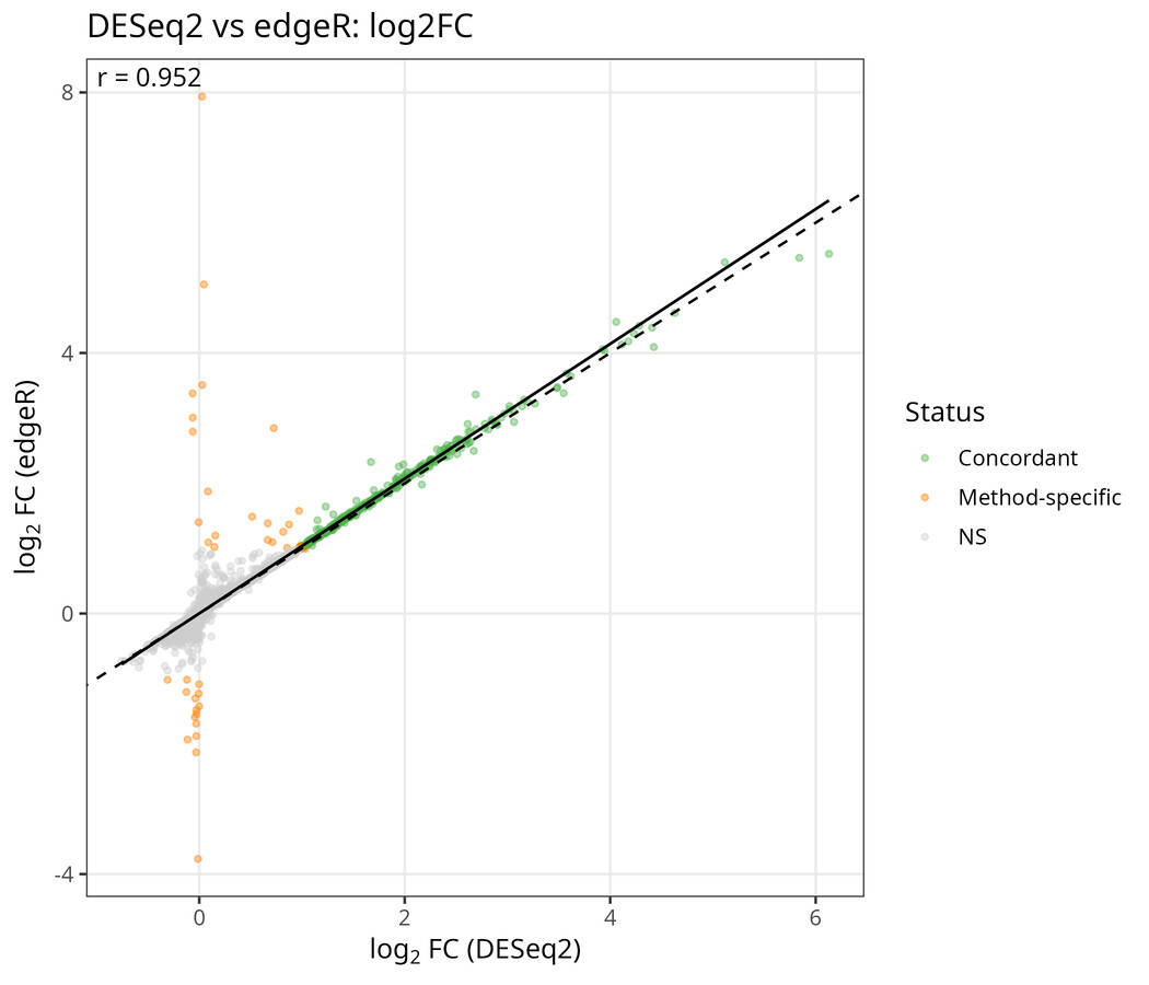 Log₂FC: DESeq2 (x) vs edgeR (y). Green = concordant significant, orange = method-specific, grey = NS. The fit (solid) nearly overlaps identity (dashed) — no systematic bias. Method-specific calls cluster near zero effect size, where edgeR is slightly less conservative (it also recovers a handful of down-regulated genes DESeq2 leaves below threshold).
This concordance is what lets you say the signal is biological rather than an artefact of one model’s assumptions. It costs little and it is the cheapest insurance in the whole pipeline.
What the Pipeline Produces
For each contrast the pipeline returns a results table (effect size, standard error, FDR), volcano and MA plots, a DESeq2-vs-edgeR concordance plot, and a heatmap of the top genes. For the 5xFAD-vs-BL6 contrast on the pooled model (~ sex + age_months + genotype + tissue, all 192 samples), the headline numbers are:
| Method | Up in 5xFAD | Down in 5xFAD | Total |
|---|---|---|---|
| DESeq2 | 418 | 0 | 418 |
| edgeR | 450 | 15 | 465 |
| Concordant | — | — | 417 |
The direction is striking and consistent: the genotype effect is almost entirely up-regulation. The top genes are an unambiguous microglial, disease-associated (DAM) signature — Trem2, Tyrobp, Cd68, Hexb, Ctsd, Clec7a, Itgax, Cst7, and the chemokines Ccl3/Ccl4/Ccl6 — exactly the program expected for amyloid-driven microglial activation in this model (Keren-Shaul et al. 2017). The near-absence of significant down-regulation in the pooled model is itself informative: a diffuse neuronal/synaptic loss is biologically expected, but pooling cortex and hippocampus and shrinking small effects pushes those modest, region-dependent decreases below threshold. That is a concrete reason the stratified analysis (below) is the natural next step rather than a formality.
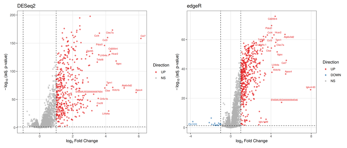 Volcano plots for 5xFAD vs BL6, DESeq2 (left) and edgeR (right), same thresholds (padj < 0.05, |log₂FC| ≥ 1). Red = up, blue = down, grey = NS. Both are dominated by the up-regulated microglial signature; edgeR additionally flags a small number of down-regulated genes (blue, left of zero) that DESeq2 leaves just below threshold. The two methods agree on the biology.
Limitations and Planned Improvements
- Region-stratified DE is the natural next analysis. The pooled model with
+ tissueis reported here and is well-powered, but it cannot expose region-specific effects or the modest down-regulation that the genotype-only-up result hints is being masked. Cortex-only and hippocampus-only contrasts (and a per-timepoint breakdown) are the logical follow-up. - No hidden-batch correction. GSE168137 was generated across many animals; surrogate-variable methods (
sva) orRUVSeqwould catch unmodeled technical structure the explicit covariates miss. - Interaction terms are underpowered. A
genotype:tissueterm is tempting but per-cell n is small; stratify-and-compare is more reliable here than one interaction model. - Multiple testing across strata. Running several region/age contrasts inflates the family-wise error; the correction needs to account for the number of contrasts, not just genes within one.
- Bulk cannot assign signal to cell types. The DAM signature is an inference from marker genes, not a measurement. Deconvolution, or the matched snRNA-seq dataset, is required to confirm it is microglia driving it.
Complementarity With Single-Nucleus RNA-seq
This dataset shares the 5xFAD model with the snRNA-seq pipeline (GSE262881). The two are complementary rather than competing: bulk RNA-seq is deep, cheap, and stable and tells you which genes and pathways move; single-nucleus resolves which cell types move but with lower per-gene sensitivity. The rigorous workflow is to use bulk to find the dysregulated programs, then single-nucleus (or deconvolution of the bulk data) to attribute them to cell populations.
Conclusion
DESeq2 is powerful only if you respect what it asks of you. Put your confounders in the design formula — and let the variance structure, not habit, tell you which ones matter (here, PC1 told us tissue could not be left out). Shrink your fold-changes, with the correct apeglm call. Cross-check against edgeR before you believe anything. On GSE168137 that discipline yields a clean, cross-validated result: 418 DESeq2 genes, 465 in edgeR, 417 concordant, almost all up-regulated, and reading as a textbook microglial/DAM signature. The combined-tissue model answers “does 5xFAD reshape the transcriptome, and in what direction” convincingly; the region-stratified analysis is the next step for “where, and what is being lost.” The methodology is not decoration — it is the reason the result is worth trusting.
Full modular pipeline and configuration: github.com/SLopezBegines/bulkRNAseq. Dataset: GSE168137.
About the author: Santiago López Begines is a PhD-trained neuroscientist and data scientist specialising in omics data pipelines, biomarker discovery, and quantitative proteomics. For scientific collaborations or methodological exchanges, get in touch.
References
Love, M. I., Huber, W., & Anders, S. (2014). Moderated estimation of fold change and dispersion for RNA-seq data with DESeq2. Genome Biology, 15(12), 550. https://doi.org/10.1186/s13059-014-0550-8
Robinson, M. D., McCarthy, D. J., & Smyth, G. K. (2010). edgeR: a Bioconductor package for differential expression analysis of digital gene expression data. Bioinformatics, 26(1), 139–140. https://doi.org/10.1093/bioinformatics/btp616
Zhu, A., Ibrahim, J. G., & Love, M. I. (2019). Heavy-tailed prior distributions for sequence count data: removing the noise and preserving large differences. Bioinformatics, 35(12), 2084–2092. https://doi.org/10.1093/bioinformatics/bty895
Forner, S., Kawauchi, S., Balderrama-Gutierrez, G., et al. (2021). Systematic phenotyping and characterization of the 5xFAD mouse model of Alzheimer’s disease. Scientific Data, 8(1), 270. https://doi.org/10.1038/s41597-021-01054-y
Keren-Shaul, H., Spinrad, A., Weiner, A., et al. (2017). A unique microglia type associated with restricting development of Alzheimer’s disease. Cell, 169(7), 1276–1290. https://doi.org/10.1016/j.cell.2017.05.018